Design of Experiments¶

"The design of experiments (DOE) also known as experiment design or experimental design, is the design of any task that aims to describe and explain the variation of information under conditions that are hypothesized to reflect the variation."

From Wiki.

In other words, the Design of Experiments (DOE) determines which experiments should be conducted to explore the parameter space of a given input/output problem.

For instance, in surrogate modeling, the goal is typically to understand the behavior of an expensive black-box function in order to make cost-effective predictions that are statistically coherent for a given input. However, as the number of dimensions in the design space increases, exploring this parameter space can quickly become overwhelming. The challenge arises because uniform exploration of a parameter space grows exponentially with the number of dimensions, a phenomenon known as the curse of dimensionality. As a result, more advanced sampling methods are often preferred over basic uniform sampling.

DoE in Melissa¶

In Melissa, sampling is handled by a parameter generator, which is initialized using the set_parameter_sampler method on the user-defined server. This method first creates a parameter_sampler instance that defines a generator method. The generator then iteratively yields parameter sets when creating client scripts.

Parameter Sampler Hierarchy¶

Melissa’s parameter sampler follows a structured class hierarchy:

At the core of this system is the BaseExperiment class, which provides essential functionalities such as defining the number of parameters, setting seeds for reproducibility, specifying parameter bounds, and implementing a generator method that calls draw. Users must implement the sample method and optionally draw to customize their parameter sampling.

The StaticExperiment class extends this functionality by allowing parameters to be stored and checkpointed, which is particularly useful for active sampling scenarios where parameters are used as foundation for producing a next set of parameters.

MixIn classes might seem complex at first, but they play a crucial role in making the implementation modular and reusable. By using MixIn classes, Melissa provides greater flexibility to create custom sampling strategies without modifying the core functionality.

How set_parameter_sampler Works¶

The set_parameter_sampler method follows these key steps:

1. Initializes a parameter_sampler instance.
2. Calls parameter_generator = parameter_sampler.generator().
3. Iterates over client scripts, retrieving parameters with list(next(parameter_generator)).
4. The generator operates as follows: generator() → draw() → sample(1).

Melissa provides predefined samplers for convenience, accessible via melissa.server.parameters.ParameterSamplerType Enums. Therefore, there are two ways in which users can register a sampler in their server class' __init__:

• By passing the Enum value to sampler_t:

  self.set_parameter_sampler(
      sampler_t=ParameterSamplerType.RANDOM_UNIFORM,
      # next are the kwargs passed to the sampler instance
      l_bounds=[-1, -1, -3]
      u_bounds=[1, 1, 3]
      seed=123
  )
  

• By passing the type of the sampler to sampler_t (See again the lorenz example):

  self.set_parameter_sampler(
      sampler_t=CustomSamplerClass,
      # next are the kwargs passed to the sampler instance
      custom_arg1=1,
      custom_arg2=3,
      ...
      l_bounds=[-1, -1, -3]
      u_bounds=[1, 1, 3]
      seed=123
  )
  

Predefined Samplers¶

Random Uniform¶

This sampler uses numpy.random.uniform when overriding the sample method.

In Melissa, users typically focus on ensemble runs, where the number of computable solutions is often large enough for uniform sampling to remain effective, regardless of dimensionality. Additionally, in sensitivity analysis, uniform sampling is particularly valuable as it provides uncorrelated samples, making it well-suited for methods like pick-freeze.

The user can instantiate RandomUniform sampler by setting:

self.set_parameter_sampler(
    sampler_t=ParameterSamplerType.RANDOM_UNIFORM
    ...
)

Scipy-based sampling¶

For deep surrogates, uniform sampling may result in slower learning due to inefficient coverage of the design space. Additionally, if training is unsatisfactory, extending the study further may be necessary. In such cases, incremental parameter space exploration can be improved using sequence sampling methods available in the scipy.stats.qmc submodule.

Halton Sequence¶

The Halton Sequence is a deterministic sampling method. In Melissa, the HaltonGenerator is based on scipy.stats.qmc Halton sampler.

The user can instantiate HaltonGenerator sampler by setting:

self.set_parameter_sampler(
    sampler_t=ParameterSamplerType.HALTON
    ...
)

Latin Hypercube Sampling (LHS)¶

The Latin Hypercube Sampling is a non-deterministic method. In Melissa, the LHSGenerator is based on scipy.stats.qmc Latin Hypercube Sampler.

The user can instantiate LHSGenerator sampler by setting:

self.set_parameter_sampler(
    sampler_t=ParameterSamplerType.LHS
    ...
)

DoE Quality Metrics¶

The Figure below compares the DOEs obtained with uniform, LHS and Halton sampling of 50 points across a parameter space of 2 dimensions:

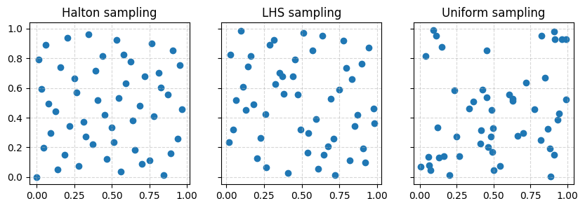
It clearly shows how uniform sampling may result in both cluttered and under-explored regions across the parameter space while Halton and LHS sampling provide a more homogeneous coverage.

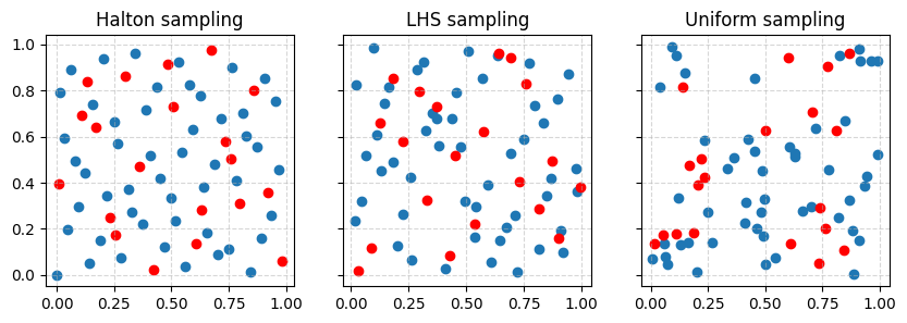
In addition, as discussed earlier, LHS and Halton sampling are sequence samplers which means that their DOE can be enhanced a posteriori by resampling from the same generator. This feature is illustrated on the figure below where 20 points are added to the previous sets of parameters.

Finally, although the quality of the DOE may seem evident from the figures, intuition may be misleading. In order to evaluate the quality of a DOE, scipy.qmc comes with a discrepancy method:

The discrepancy is a uniformity criterion used to assess the space filling of a number of samples in a hypercube. A discrepancy quantifies the distance between the continuous uniform distribution on a hypercube and the discrete uniform distribution on distinct sample points.

The lower the value is, the better the coverage of the parameter space is.

For the DOEs represented in this section, the following discrepancies were obtained: